Distribution and Regime Effects in a 1DTE Options Strategy
Motivation
Short-dated premium strategies are popular because they win often. Selling very short-dated options on indices like SPX can produce a steady stream of small gains, and the resulting equity curves can look stable for long stretches of time. However, that stability can be misleading. Rather than indicating genuine edge, it can mask asymmetric tail risk. Here I implement a deliberately naive version of the strategy in order to analyze when and where it breaks down.
Strategy & Backtest Description
The strategy trades a 1 day-to-expiration (DTE) iron condor on the SPX. It’s simple and rule-based with no parameter tuning beyond sensible defaults. Each trade uses fixed 20-point wide spreads that caps maximum risk and targets a total credit between 1.05 and 1.45. Short puts are selected with deltas between 2 and 10, and short calls between 2 and 8 with a few constraints to keep credit and delta roughly balanced between the two sides.
In general, trades are entered toward the end of the trading session at 3:50pm ET. However, if the next day is an FOMC rate decision, CPI release, unemployment report, then the trade is skipped in order to avoid known tail risk events. The exit rules are mechanical. Before 12:00pm the trade exits on 0DTE if it reaches 60% of profit or its price reaches three times premium received. After 12:00pm on 0DTE the trade will exit if at all profitable. Finally, after 1:00pm the trade will exit regardless.
This strategy is backtested from April 1, 2022 (when daily expirations first became available on SPX) through December 31, 2025. The portfolio starts with $50,000. This amount ensures sufficient capital to avoid forced liquidations and allow trades to evolve according to their defined exit rules. Only one iron condor is entered per trade (short one call spread and one put spread) with no scaling or compounding. Thus, the capital is not fully deployed and the system used only the margin required for a single position at a time. Transaction costs are included using QuantConnect’s Schwab brokerage model and orders are assumed to fill immediately with no slippage. The backtest operated on hourly data to capture intraday path dynamics relevant to stop-loss and time-based exits.
Results
The strategy executed 717 trades with an overall win rate of 82.57%. Despite this high win frequency, the expectancy per trade was −0.078, and the portfolio finished the test period down approximately $5,540 (excluding fees). The summary statistics are reported in Summary Metrics table. The combination of a high win rate and negative expectancy suggests payoff asymmetry. The small, frequent gains were offset by fewer, large losses.
| Summary Metrics | Worst Trades | Value | Month | |||||
|---|---|---|---|---|---|---|---|---|
| Total Trades | 717 | Expectancy (per trade) | -0.078 | Skewness | -3.08 | -15.9 | 2025-04 | |
| Wins | 592 | Average Win | 0.853 | Kurtosis | 9.98 | -14.5 | 2024-07 | |
| Losses | 125 | Average Loss | -4.482 | Fees | $5732 | -13.95 | 2023-05 | |
| Win Rate | 82.57% | Total PnL | -55.40 | -12.45 | 2025-01 | |||
| -11.9 | 2023-09 |
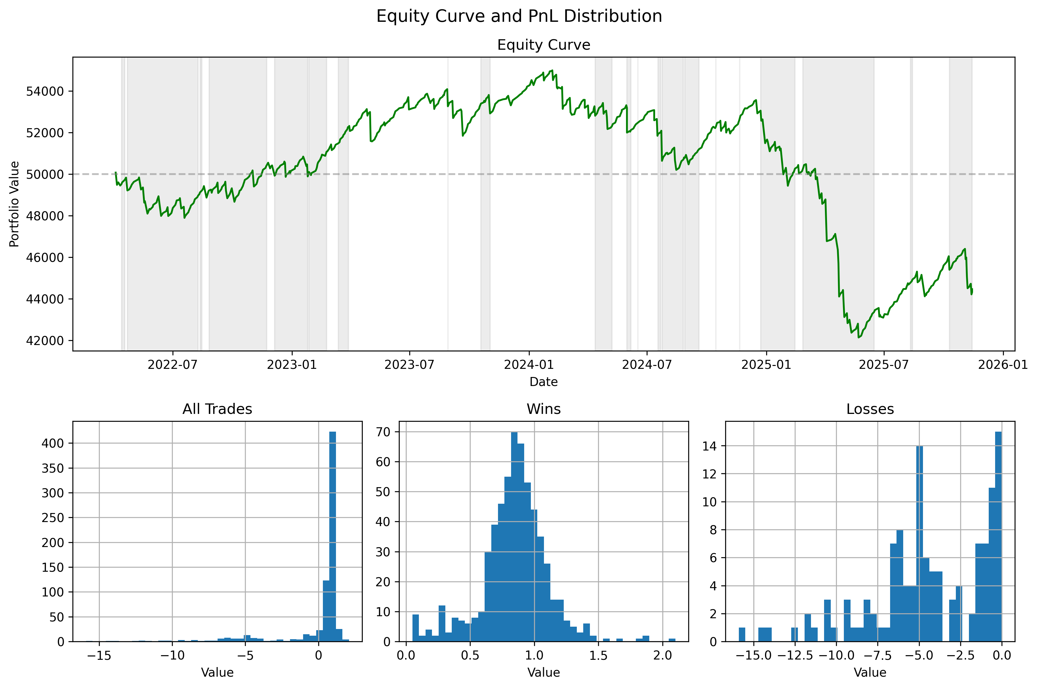
The PnL distribution above illustrates this structure. The wins are tightly clustered while losses have a pronounced fat left tail. This asymmetry is reflected in the negative skew (−3.08) and elevated kurtosis (9.98). The heavy tail risk is demonstrated by the worst trades shown in Worst Trades table above. They illustrate the magnitude of these tail events. The equity curve plot above reinforces this pattern visually. There are periods of stability, but they are punctuated by sharp drawdowns during regime deterioration. Taken together these results indicate the performance is dominated by tail risk even though the strategy wins often.
Analysis
The starting point is the trade PnL distribution. Although the strategy wins more than 82% of the time, its negative expectancy is driven by a small number of extreme outcomes. Removing the worst ten trades flips expectancy from −0.078 to 0.042. This isn’t a solution, but it does suggest that the strategy isn’t steadily eroded by frequent small losses. Rather, performance is dominated by rare and large drawdowns. In normal conditions, the system behaves profitably, but under stress, losses overwhelm gains.
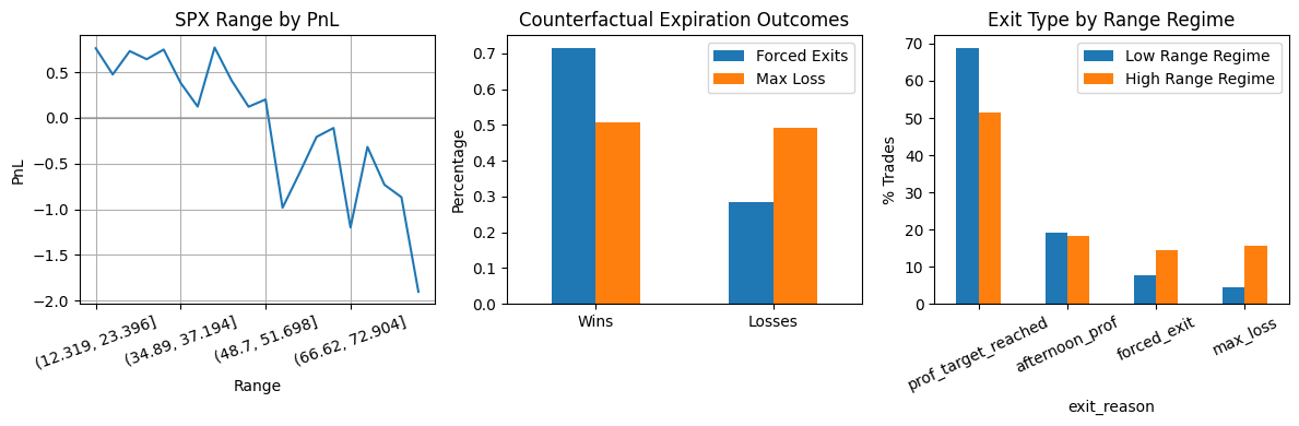
To understand when these large losses occur, I partitioned trades by intraday SPX range (first chart above). A break appears around 51 points. Below that threshold, the strategy is strongly profitable: 394 trades with a 90.6% win rate and a mean PnL of 0.489, producing 192.75 in total PnL. Above that threshold, the regime reverses. The 323 trades in this range show a 72.7% win rate and a mean PnL of −0.768, producing −248 in total PnL. These metrics are summarized in the table below. The change in expectancy is not gradual. It flips sign indicating a structural regime shift rather than a smooth deterioration.
| Regime | Trade Count | Win Rate | Mean PnL | Avg Win | Avg Loss | % Max Loss Exits | Total PnL |
|---|---|---|---|---|---|---|---|
| Range $<$ 51.698 | 394 | 0.906 | 0.489 | 0.841 | -2.909 | 0.046 | 192.75 |
| Range $\geq$ 51.698 | 323 | 0.727 | -0.768 | 0.87 | -5.144 | 0.158 | -248 |
The difference isn’t just in average returns. The exit mechanics shift as well. The Exit Type by Range Regime plot shows that in the low-range regime, only 4.6% of trades hit the max-loss condition. In the high-range regime, that figure rises to 15.8%, while profit-target exits fall materially. The structure of exits changes when range expands. This directly links intraday range to stop-loss activation, not merely to realized PnL. The degradation in performance during high-range periods follows from how the strategy responds to large intraday moves.
The counterfactual exit analysis sharpens this further (middle plot above). Roughly 50% of max-loss trades would have expired profitably if held to expiration. For forced exits, nearly 70% would have recovered. Realized losses therefore aren’t purely a function of where the market closes. They are heavily influenced by how price moves during the day. The stop-loss reduces true terminal blow-ups, but it also locks in temporary intraday drawdowns. The loss engine is not simply “short gamma loses on volatile days.” It is the interaction between volatility regime shifts and rule-based exits that converts intraday instability into realized losses.
In sum, the strategy doesn’t appear uniformly unprofitable. It is profitable in calm regimes and structurally fragile during sustained intraday range expansion. The long-run outcome is determined by how often the market enters that second regime.
Conclusions
The core insight from this baseline strategy is that a high win rate can conceal structural exposure to large losses. The strategy is profitable in calm regimes where intraday range remains contained, but performance deteriorates sharply once range expands beyond a clear threshold. In those high-range regimes, stop-loss and forced exits trigger more frequently, and a meaningful fraction of those trades would have recovered by expiration. This shows that losses are not simply a function of terminal payoff, but of how intraday volatility interacts with rule-based exits. The strategy is not continuously unprofitable. It’s profitable in stable conditions and structurally fragile during intraday range expansion.
A natural question that follows from this analysis is whether high intraday range regimes are predictable at the time of entering a trade. Are there observable market conditions that contain information about the probability of next-day range expansion? If variables such as VIX level, VIX term structure (comparing VIX1D, VIX9D, VIX), overnight gaps, prior day’s realized range, or implied versus realized volatility spreads meaningfully increase the likelihood of entering a high-range regime, then the strategy’s fragility may be managed through conditioning or trade filtering. If they don’t, then the regime behavior identified above represents structural exposure to unpredictable intraday shocks rather than a manageable risk.