Forecasting Intraday Regime Risk in a 1DTE SPX Strategy
Motivation
I analyzed a simple 1-day-to-expiration (1DTE) SPX iron condor strategy in a previous post. I found that the strategy is not uniformly unprofitable. Rather, its performance depends heavily on the intraday volatility regime. On calm days the system performs well, but on days with large intraday ranges the strategy becomes fragile. The majority of losses occur when stop-loss rules trigger during large intraday swings, and many of those trades would have expired profitably if they had simply been held to expiration.
The baseline strategy itself is intentionally simple. Each trade sells a 1DTE SPX iron condor with 20-point wide spreads targeting roughly $1.05–$1.45 in premium. Trades are entered near the close (3:50pm ET) and exit rules are mechanical, based on profit targets, stop losses, and time-based exits the following day. The system trades only one position at a time and skips known macro event days such as FOMC or CPI releases. When I backtested the strategy from April 2022 through December 2025, it produced a high win rate but negative overall expectancy due to a small number of large losses. Those losses are closely tied to the size of the intraday range. A summary of strategy’s statistics is in the table below.
| Regime | Trade Count | Win Rate | Mean PnL | Avg Win | Avg Loss | % Max Loss Exits | Total PnL |
|---|---|---|---|---|---|---|---|
| Range < 51.698 | 394 | 0.906 | 0.489 | 0.841 | -2.909 | 0.046 | 192.75 |
| Range ≥ 51.698 | 323 | 0.727 | -0.768 | 0.87 | -5.144 | 0.158 | -248 |
The strategy performs well when the SPX stays within a relatively small range. But when the range exceeds roughly 52 points, the strategy loses money on average. Given this behavior, I wanted tot answer the questionL: Can we estimate the probability that tomorrow will be a high-range session at the time the trade is entered? If that probability can be forecast with reasonable accuracy, then it might be possible to condition the strategy by filtering trades, adjusting position size, or modifying exit rules. To formalize this, I treat the next day’s range regime as a latent state variable:
\[Y_{range}(t) = \begin{cases} 1 & \text{if next-day SPX intraday range} \ge 51.698 \\ 0 & \text{otherwise} \end{cases}\]Tomorrow’s range is unknown at the time the trade is opened. So the goal of this post is to determine whether the probability of that regime can be estimated using information available at entry.
Experimental Setup
All data for the experiments is sourced from QuantConnect. I pulled daily SPX, VIX, and VIX9D prices from April 2022 through December 2025 which covers the entire modern period of daily SPX options expirations. The target variable is the next day’s intraday range relative to the threshold identified in the analysis of the baseline strategy. Several potential predictors were constructed from both realized and implied volatility measures.
The following features attempt to capture both recent market behavior directly from SPX price movements. These features tested whether recent market volatility and shocks contains signal about the next day’s range:
- Prior day intraday range
- 5-day average range
- Prior day absolute return
- Overnight gap magnitude
I also tried to capture the market’s expectations of volatility through volatility indices. These features tested whether the volatility market’s expectations contains signal about the next day’s range:
- Prior VIX close
- Prior VIX9D close
- The slope between the two
I split the dataset chronologically to preserve the time-series structure of the problem. The training dataset consists of daily price observations from April 2022 to December 2023 and the test dataset covers January 2024 to December 2025.
I evaluated models using three metrics: log loss, Brier score, AUC (area under curve). In general, these metrics capture two different aspects of the performance: ranking ability and the accuracy of the forecasted probabilities. The log loss is used to determine how well the predicted probabilities match realized outcomes. Incorrect but confident predictions are penalized which favors well-calibrated probability forecasts. The Brier score is essentially the mean squared error of predicted probabilities. It evaluates the quality of the probability estimates themselves rather than just the ranking. And the AUC measures ranking quality. It evaluates whether the model assigns higher probabilities to high-range days than to low-range days regardless of the exact probability values.
I also examined lift tables and calibration curves. The lift tables buckets predictions into probability groups and compare predicted probabilities to actual outcomes. The calibration curves plot predicted probability against realized frequency and reveal whether forecasts are systematically too aggressive or too conservative.
Summary of Results
The experiments evaluated four different feature sets to determine which predictors help forecast whether the next day’s SPX intraday range will exceed the regime threshold at trade entry. A summary of the log loss, Brier score, and AUC is in the table below. Log loss and Brier score measure the accuracy of the probability forecasts and AUC measures how well the model ranks high-range versus low-range days.
| Feature Set | Log Loss | Brier | AUC |
|---|---|---|---|
| Realized Vol | 0.606 | 0.201 | 0.746 |
| Implied Vol | 0.668 | 0.234 | 0.789 |
| Combined | 0.614 | 0.213 | 0.777 |
| Final Regime Features | 0.574 | 0.193 | 0.775 |
Several patterns stand out. The realized volatility features produce the best ranking performance, reflected in their AUC score. However, the implied volatility features alone perform worse in terms of probability accuracy, suggesting that the volatility indices by themselves do not capture the short-term regime shifts relevant to this strategy. Combining realized and implied volatility improves results slightly, but the largest improvement comes from adding two shock variables: overnight gap magnitude and prior absolute return. The final feature set (5-day average intraday range, prior VIX/VIX9D slope, overnight gap magnitude, and prior absolute return) achieves the best log loss and Brier score, indicating that it produces the most accurate probability forecasts.
In order to arrive at the final feature set, I performed ablation tests by removing each feature one at a time to better understand which features drive the signal. The most important variable is clearly the 5-day average range. Removing it causes log loss to deteriorate substantially, indicating that recent realized volatility state is the strongest predictor of the next day’s regime. The shock variables (prior absolute return and overnight gap magnitude) also contribute meaningful signal. Removing either of them weakens the model. Interestingly, implied volatility variables appear largely redundant once realized volatility is included. Removing VIX or VIX9D features barely changes the model’s performance.
| Feature Set | Log Loss | Brier | AUC |
|---|---|---|---|
| All features | 0.597 | 0.207 | 0.790 |
| w/o prior_vix_close | 0.593 | 0.205 | 0.790 |
| w/o prior_vix9d_close | 0.594 | 0.206 | 0.790 |
| w/o prior_slope | 0.596 | 0.206 | 0.790 |
| w/o 5d_avg_range | 0.648 | 0.227 | 0.803 |
| w/o prior_range | 0.588 | 0.204 | 0.800 |
| w/o prior_abs_ret | 0.603 | 0.209 | 0.786 |
| w/o gap_mag | 0.606 | 0.210 | 0.781 |
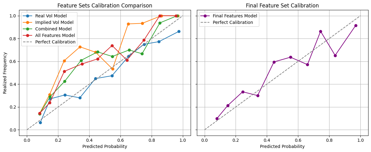
The calibration curves below illustrate how the probability forecasts evolve as features are added and removed. The realized volatility features tend to produce conservative forecasts, while the implied volatility features appear unstable across probability buckets. The combined features produce more stable forecasts, and the final feature set generates the most consistent probability estimates overall.
 \
\
Focusing on the final feature set, the lift table shows a clear monotonic relationship between predicted probability and realized outcomes. The highest risk bucket contains far more high-range sessions than the lowest bucket, indicating that the model meaningfully separates calm and volatile regimes.
| Quintile | Mean Probability | Realized Frequency | Count |
|---|---|---|---|
| 0 | 0.12 | 0.19 | 101 |
| 1 | 0.21 | 0.29 | 100 |
| 2 | 0.33 | 0.33 | 100 |
| 3 | 0.57 | 0.62 | 100 |
| 4 | 0.90 | 0.84 | 100 |
Analysis
The experimental results contain several clear patterns.
First, realized volatility carries the strongest predictive signal. The ablation tests show that the 5-day average range is the dominant feature. Removing this feature causes the largest deterioration in performance by a wide margin indicating that the recent realized volatility state of the market carries substantial information about the following day’s intraday range. This result is consistent with a well-known property of financial markets: volatility clusters over time. Periods of elevated volatility tend to persist making recent realized volatility a strong predictor of near-term volatility regimes.
Second, recent price shocks add meaningful information. The two additional features added to the final model (prior day absolute return and overnight gap magnitude) improve the model’s forecasting accuracy. These features capture sudden or abnormal price movements. Large shocks appear to increase the probability that the next day will have a large intraday range. These shock features likely work because they reinforce volatility clustering. Large price moves often trigger position adjustments, hedging flows, and liquidity imbalances that can persist into the following day. In effect, a large move today increases the probability of another volatile session tomorrow. These features complement the realized volatility features by capturing short-term disturbances in market.
Third, somewhat surprisingly, the implied volatility adds limited signal. The implied volatility features contribute relatively little predictive power once realized volatility is included. Removing VIX and VIX9D features in the ablation tests produces almost no change in model performance. One interpretation is that the information contained in implied volatility is quickly reflected in realized price behavior. So, once recent SPX volatility is included in the model, the volatility indices add little additional information about near-term volatility regimes.
Fourth, the results also highlight the difference between the evaluation metrics. The realized volatility model achieves the highest AUC meaning it’s better at ranking which days will have higher or lower ranges. However, the final feature set produces much lower log loss and Brier score. So the final features generate more accurate probability estimates. This distinction matters because the ultimate objective of the model is to decide whether to enter a trade. Thus, the calibration of the probability estimates of entering a hostile regime is more important than ranking alone. A well-calibrated probability forecast allows the strategy to apply and adjust thresholds, e.g. skipping trades when regime risk exceeds a certain level.
Fifth, the model meaningfully separates regimes. The lift table confirms that the model produces a monotonic lift across probability buckets. As predicted probability increases, the realized frequency of high-range sessions also increases. This monotonic relationship is important because it meaningfully stratifies trading days by regime risk. This means the model’s forecasts can potentially be used to condition trading decisions. If the predicted probability of a hostile regime is high, then the strategy could reduce exposure, skip the trade, or adjust exit logic.
In sum, these results demonstrate that the probability of entering a high-range session contains measurable structure rather than being purely random. Recent volatility conditions and recent price shocks both provide useful information about the following day’s regime. This does not mean the model perfectly predicts future volatility regimes, but it does suggest that the strategy’s exposure to large intraday moves is at least partially predictable.
Conclusion
The main result of the experiments and analysis is that next-day intraday range regimes contain measurable structure and can be partially forecast using information available at trade entry. A relatively simple feature set built from recent realized volatility and recent market shocks produces calibrated probability forecasts that stratify trading days into meaningfully different levels of regime risk. In other words, the model meaningfully separates days that are likely to be calm from days that are more likely to experience large intraday moves. This does not mean the forecast is perfect. But it does suggest that the strategy’s vulnerability to high-range days is not purely random. So, instead of viewing the system as structurally fragile, it’s more accurate to think of it as conditionally fragile. This conclusion raises the question that matters most for traders: Do these probability forecasts actually improve the strategy’s economic performance? If the model can reliably identify risky regimes, then the strategy might benefit from filtering trades, adjusting exposure, or modifying exit behavior during those periods. In a future post I’ll incorporate these regime forecasts directly into the trading system to test whether filtering or conditioning trades based on predicted risk improves the strategy’s PnL.