Some Notes on Short-Term SPX Vol
Motivation
I’ve been looking more closely at short-vol carry trades on the SPX. These trades try to collect a small premium with a high win rate and occasional losses. A common explanation for why they work is that implied volatility (IV) is often “too high” and realized volatility (RV) ends up being lower. In other words, the IV distribution is generally wider than the RV distribution. So expectations about future moves tend to be broader than what actually occurs.
My analysis here doesn’t include option prices. So it doesn’t establish whether the premium is sufficient. It only shows that the implied distribution is generally wider than realized. However, to make it more concrete, I also model a simple iron condor. At each entry, I place the short strikes at 1.5 standard deviations (based on implied volatility) away from the spot price. A trade is considered a win if neither short leg expires in the money.
As a quick aside, you might consider why someone would consistently take the other side of this trade if they’re regularly overpaying and frequently losing. These counterparties are generally not optimizing this trade in isolation. Rather, this trade is typically part of a larger strategy in which they are operating under constraints (hedging, risk limits, event exposure). For example, they may need to buy short-term protection, manage gamma exposure, or position around specific events. So, given this perspective, overpaying slightly for short-dated options can be rational. The objective is not to maximize the expected value of a single trade, but to satisfy broader portfolio or risk requirements.
Setup
In order to generate a dataset to compare the implied volatility with realized volatility I started with the VIX9D as a proxy for implied volatility over the next nine days. I then compute the forward nine day realized volatility from SPX log returns so that implied and realized measures are directly comparable. I define the IV-RV spread as the difference between the VIX9D measure and the forward realized volatility of the SPX. I also compute a three day rolling RV average as a simple backward-looking measure of recent market behavior. Finally, using the implied volatility, I estimate the expected move and place short strikes at roughly 1.5 standard deviations from spot. I then check how often these strikes would have expired in the money.
A notebook with these calculations and the results can be found here along with the data here.
Results
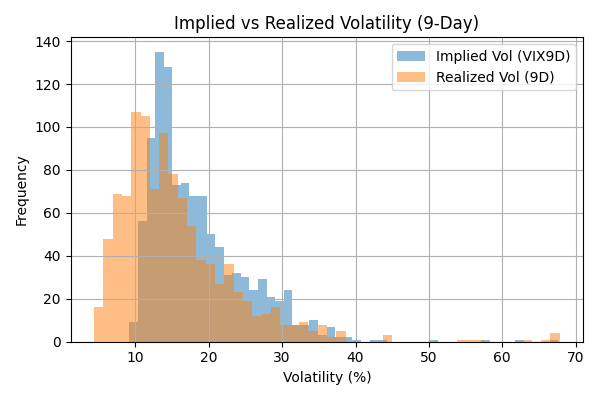
The core observation is that the IV is generally higher than RV. On average, the implied distribution is wider than what actually occurs (see the histogram below). This is consistent with IV exceeding the forward RV in roughly 80% of observations which aligns with the intuition behind short-vol trades.
This relationship is also reflected in the volatility averages (Table: Vol Averages). IV is nearly identical between winning and losing trades, but RV is significantly higher in the losing cases. As a result, the IV–RV spread is positive for wins and strongly negative for losses.
| Vol Averages | Wins(n=1039) | Losses(n=18) |
|---|---|---|
| iv | 18.553 | 18.798 |
| rv | 15.335 | 28.242 |
| iv_rv_spread | 3.218 | -9.444 |
| iv_rolling_rv_spread | 3.897 | 3.668 |
Another observation is that the cases where the RV exceeds what’s implied are not gradual, but sudden. Backward-looking realized volatility provides little information about whether the next trade will succeed. This can be seen by comparing the win rates of the spread buckets in the below table. When grouping by the IV–RV spread, the win rate increases monotonically as the spread widens. This suggests that when IV is more overstated relative to what actually occurs, outcomes improve. In contrast, when grouping by IV relative to trailing RV, win rates remain relatively flat across buckets. This indicates that trailing RV provides little useful information at trade entry.
| iv_rv_spread buckets | Win Rate | iv_rolling_rv_spread buckets | Win Rate |
|---|---|---|---|
| (-45.34, 0.791] | 0.936 | (-47.522, 0.64] | 0.989 |
| (0.791, 3.605] | 0.996 | (0.64, 4.489] | 0.970 |
| (3.605, 6.275] | 1.0 | (4.489, 7.518] | 0.981 |
| (6.275, 24.0] | 1.0 | (7.518, 25.811] | 0.992 |
Trade failures occur when realized volatility expands sharply. In the loss cases, realized volatility jumps dramatically relative to implied volatility (Table: Vol Averages). These are not slow breakdowns but sudden shifts that are usually tied to discrete events. A geopolitical shock like we’ve had this year, for example, can quickly push realized volatility far beyond what was implied. The IV–RV spread buckets support this point. As the spread increases, the win rate approaches 100%. When the implied distribution is sufficiently wide relative to realized outcomes, the short strikes are unlikely to be breached.
In sum, the market does overestimate the IV relative to realized outcomes. Failures are driven by sudden expansions in realized volatility rather than gradual changes, and the degree of overstatement matters: larger IV–RV spreads correspond to higher containment rates.
Summary
The above analysis doesn’t incorporate option prices. So it doesn’t directly measure profitability or whether the premium is sufficient. It only shows that the implied distribution is regularly wider than the realized distribution, and how that relates to the short strikes on a hypothetical iron condor being breached. The key points that the analysis demonstrates are that:
- The market tends to price a broader distribution of moves than what actually occurs.
- The trades fail when RV expands rapidly beyond what was implied and not because conditions were slowly deteriorating.
- The trailing RV provides little information about whether the next trade will succeed.
My key takeaway from this analysis is that short-vol carry trades can be reasonable not by trying to predict the market, but rather by consistently operating in a context where expectations are often broader than reality so long as risk is managed when that relationship breaks down. So these trades rely more on pricing and risk management rather than forecasting. You can’t reliably forecast the next shock event. But you can observe how IV and RV are behaving relative to each other. For example, plotting IV against RV (and their rolling averages) provides a simple way to see when the market is pricing a wider or narrower distribution than what is being realized. When the two move together, pricing is roughly in sync. When they diverge, the implied distribution is either expanding or compressing relative to actual outcomes.